Solving quadratic equations (equations that can be written in the form ax2 + bx + c = 0, where a ≠ 0) is a major topic in high school Algebra. Typically, students in the U.S. learn several methods to solve them (factoring, graphing, completing the square, or using the quadratic formula). In my experience, many students not only struggle to learn four very different methods but then have to contend with determining which method works best for a given quadratic equation.
A few months ago, mathematician Po-Shen Loh published an article and video online (both can be viewed at http://www.poshenloh.com/quadratic/) that described a different way to solve quadratic equations. Although he devised it independently, other mathematicians, including the ancient Babylonians and Greeks as well as John Savage in a 1989 Mathematics Teacher article, developed similar techniques (Loh describes them in more detail at http://www.poshenloh.com/quadraticrelated/).
This year, I teach an Algebra I class of high school freshmen and sophomores, many of whom are repeating the course. I decided to teach the method outlined by Loh to my students. Along the way, I made several modifications to accommodate my students’ needs, the most notable of which was to add a visual element to the method to help students remember and understand the steps. This article describes the lessons that I would use to teach what I call the mean-product method and how students reacted to it. (These descriptions reflect modifications that I made after initially teaching these concepts.)
Lesson 1: Understanding the Graph of a Quadratic Function
To understand how to solve quadratic equations, students should be familiar with the characteristics of the graphs of quadratic functions. Since many of my students had already seen these graphs before, I was able to quickly review many of their characteristics. If I were teaching students who had not seen quadratic functions before, I would introduce this with an activity in which students work in groups of two or three to graph several quadratic functions using technology and note their equations in standard and factored form as well as their x-intercepts, the sum of the x-intercepts, and the product of the x-intercepts. This could be done with a table like Table 1 below:
| Equation (factored form) | Equation (standard form) | Sketch of graph | Equation of axis of symmetry | x-intercepts | Sum of x-intercepts | Product of x-intercepts |
| (x – 2)(x – 8) = 0 | x2 – 10x + 16 = 0 | x = | ||||
| (x – 4)(x – 3) = 0 | x2 – 7x + 12 = 0 | x = | ||||
| (x + 1)(x – 5) = 0 | x2 – 4x – 5 = 0 | x = | ||||
| … | … | … | … | … | … | … |
Table 1. Characteristics of Quadratic Equations
Since students haven’t learned factoring yet, I would give them the equations in both standard and factored form. To simplify this task, a = 1 in all cases here. The goal here is for students to be able to determine the sum and product of the x-intercepts as well as the equation of the axis of symmetry given the equation in standard form.
Lesson 2: Summarizing the Characteristics of a Quadratic Function
After the previous lesson, students should reach the following conclusions (all of which are critical for solving quadratic equations) for the equation y = ax2 + bx + c:
- The x-intercepts of the graph are the opposites of the numbers in the factored form of the polynomials.
- The axis of symmetry is located midway between and is the average of the x-intercepts.
- The sum of the x-intercepts is half of the opposite of b.
- The product of the x-intercepts is equal to c.
Students may struggle to use the correct terminology (they may say something like “the number in parentheses flips with the sign in the answers”). To encourage students to brainstorm, I allow them to use informal language at first. After students make their observations, I introduce some terminology to help students describe their thinking me precisely:
- The zeros of a function f are the x-values that make the equation f(x) = 0 true (in other words, that lead to an output of 0).
- The x-intercepts of the graph of a function are the points where the graph crosses the y-axis.
- The roots of an equation are the values of the variable that make it true.
Students should not refer to the “zeros of a graph” or “roots of a function.” Functions have zeros, graphs have x-intercepts, and equations have roots. However, all of these terms are related. To emphasize this vocabulary, I would even spend a lesson or part of a lesson doing examples in which students fill in the blanks in sentences using the proper terms. For example:
1. Fill in the blanks with the correct words: The __________ of the __________ y = (x – 3)(x + 4) are 3 and –4.
SOLUTION: The zeros of the function y = (x – 3)(x + 4) are 3 and –4.
2. Fill in the blanks with the correct words: The __________ of the __________ y = (x + 5)(x – 6) are (–5, 0) and (6, 0).
SOLUTION: The x-intercepts of the graph of y = (x + 5)(x – 6) are (–5, 0) and (6, 0).
3. Fill in the blanks with the correct words: The __________ of the __________ (x + 12)(x + 13) = 0 are –12 and –13.
SOLUTION: The roots of the equation (x + 12)(x + 13) = 0 are –12 and –13.
In this lesson, students should also complete a table similar to Table 2 so that they become more familiar with the characteristics of quadratic functions given their graphs or equations. This table can contain equations in factored form so that students can multiplying polynomials (preferably using the box or area model, which I wrote about at http://bobsonwong.com/blog/21-think-inside-the-box-2).
| Equation (factored form) | Equation (standard form) | Sketch of graph | Equation of axis of symmetry | x-intercepts | Sum of x-intercepts | Product of x-intercepts |
| y = (x – 1)(x – 5) | x = | |||||
| x = | 2, 6 | |||||
| y = x2 – 12x + 20 | x = 6 | 12 | 20 | |||
| … | … | … | … | … | … | … |
Table 2. Filling in the Characteristics of Quadratic Functions
Lesson 3: Determining the Characteristics of a Quadratic Function from Its Graph
In the next lesson, students need to determine the characteristics of a quadratic function given other characteristics. Students should work through graphs of quadratic functions labeled with various characteristics and asked them to find the missing characteristics, labeled as variables. Below are some examples.
4. Find the values of u and m:
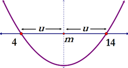
SOLUTION: Students are given the x-intercepts and asked to find their average (m) and the distance between the average and each root (u). Here, x1 = 6 – 2 = 4 and x2 = 6 + 2 = 8. After doing several examples with positive roots, students should work through examples with a positive and negative root as well as examples with two negative roots.
5. Find the values of x1 and x2:
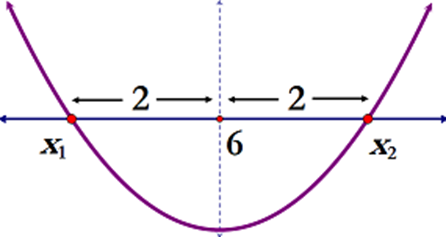
SOLUTION: Students are given the equation of the axis of symmetry (x = 6), which corresponds to the average of the x-intercepts, and they are asked to find the x-intercepts, which are labeled x1 and x2. The graph shows that x1 = 6 – 2 = 4 and x2 = 6 + 2 = 8. Again, students should also work through other examples with positive and negative roots.
Lesson 4: Determining the Zeros of a Quadratic Function Given Their Product and Average
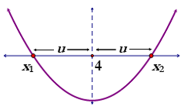
6. Find the values of u, x1, and x2:
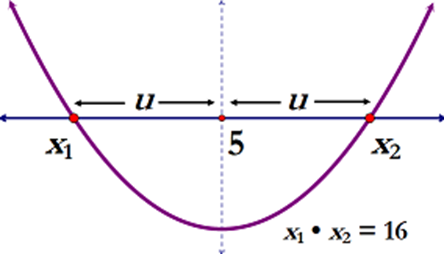
SOLUTION: Students are given the average and the product of the x-intercepts and are asked to find the x-intercepts. They should see from the graph that the x-intercepts are x1 = 5 – u and x2 = 5 + u. They can write an equation that expresses the product of the x-intercepts in two ways:
x1 · x2 = 16
(5 – u)(5 + u) = 16
25 – u2 = 16, so u2 = 9, or u = 3.
(NOTE: Although u = ±3, we may ignore the negative root since the graph is symmetrical and the roots are x = 5 ± u.)
Thus, x1 = 5 – u = 5 – 3 = 2 and x2 = 5 + u = 5 + 3 = 8.
This slightly simplified version of the method described by Loh leads to the next lesson, in which students start solving quadratic equations.
As they did in Lesson 3, students here should also do several examples with all positive, positive and negative, and all negative roots.
Lesson 5: Solving Quadratic Equations with a = 1 and Integral Roots
In this lesson, students solve quadratic equations in which a = 1 and the roots are integers. This lesson will work best if the product of the roots is sufficiently large so that students can’t easily guess the factors, such as:
7. Solve for x: x2 – 20x + 96 = 0.
SOLUTION: I strongly recommend that students sketch a graph like the one below to solve these problems.
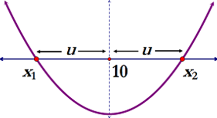
From the previous lesson, students should be able to reach the following conclusions from the equation:
- The sum of the roots is –b = –(–20) = 20.
- The average of the roots (i.e. the sum of the roots divided by 2) is 20/2 = 10.
- The product of the roots is c = 96.
Here’s where this method really saves time. Using the commonly taught “guess-and-check” method, students must find the two numbers that multiply to 96 and add to 20. This can be tedious and frustrating! This method provides a more systematic procedure. From the graph, we see that the roots are x1 = 10 – u and x2 = 10 + u. Students can write an equation that expresses the product of the roots in two ways:
x1 · x2 = c
(10 – u)(10 + u) = 96
100 – u2 = 96, so u2 = 4, or u = 2.
Thus, x1 = 10 – u = 10 – 2 = 8 and x2 = 10 + u = 10 + 2 = 12.
Lesson 6: Solving Quadratic Equations with a = 1 and Fractional Averages
Sometimes, the roots will have fractional averages, such as the following:
8. Solve for x: x2 – 21x + 98 = 0.
SOLUTION:
From the equation, we see that the sum of the roots is –b = –(–21) = 21, so the average of the roots is 21/2. In addition, the product of the roots is c = 98. From the graph, we see that the roots are x1 = 21/2 – u and x2 = 21/2 + u.
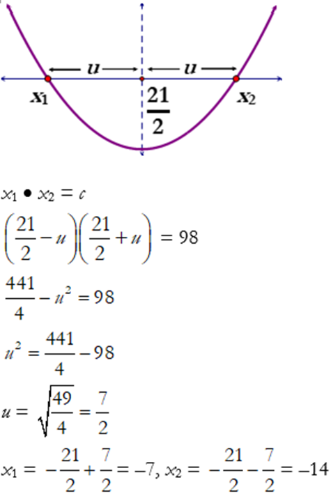
Although this may seem like a concept that can be incorporated into the previous lesson, I found that taking an extra day helped students get comfortable with the ideas underlying this method. In addition, many students are uncomfortable with fractions, so this lesson gives students more time and practice.
Lesson 7: Solving Quadratic Equations with a = 1 and Irrational Roots
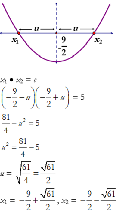
In the next lesson, students solve quadratic equations with irrational roots, such as the following:
9. Solve for x: x2 + 9x + 5 = 0.
SOLUTION:
Lesson 8: Solving Quadratic Equations with a ≠ 1
In this lesson, students solve quadratic equations in which a ≠ 1. For these problems, students must first divide the entire equation by a. This will make the problem more challenging than previous ones, but I found that students who struggle with fractions can use a calculator to perform operations with fractions (most graphing calculators can be configured to convert the result into a fraction in lowest terms) or convert them the fractions into decimals.
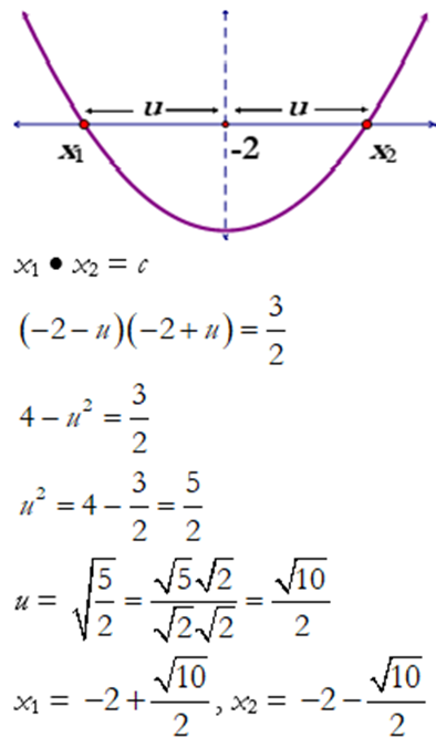
10. Solve for x: 2x 2 + 8x + 3 = 0.
SOLUTION: Dividing the equation by a = 2 gives us x2 + 4x + 3/2 = 0. Here, the average of the roots is –4/2 = –2 and the product is 3/2.
Lesson 9: Solving Quadratic Equations with Imaginary Roots
For students who have to solve equations with imaginary roots (in New York State, where I teach, these equations are taught in Algebra II, not Algebra I), the next lesson would include questions like the following:
11. Solve for x: x2 – 8x + 17 = 0.
SOLUTION:
x1 · x2 = c
(4 – u)(4 + u) = 17
16 – u2 = 17
u2 = –1
u = i
x1 = 4 + i, x2 = 4 – i
Since the roots are imaginary, the graph has no x-intercepts, so the horizontal line here is not the x-axis. I wondered what the points x1 and x2 represent graphically, so I did some research on graphing complex roots on quadratic equations. This visualization of the complex roots requires graphing quadratic equations in three dimensions, with the z-axis representing imaginary numbers. Fortunately, I found several references:
- The Math Department at Queen’s College in Hong Kong explains a procedure for finding the complex roots in the real coordinate plane: http://www.qc.edu.hk/math/Advanced%20Level/Complex%20roots.htm
- Aran Glancy created a Geogebra animation that visualizes complex roots of quadratic equations in three dimensions: http://www.geogebra.org/m/U2HRUfDr
- Carmen Artino published an article in Parabola (2009) explaining how to graph the complex roots of a quadratic equation: http://www.parabola.unsw.edu.au/2000-2009/volume-45-2009/issue-3/article/complex-roots-quadratic-equation-visualization
- Joseph Pastore and Alan Sultan at Queens College, City University of New York published an article explaining a geometric interpretation of complex zeros of quadratic functions: http://geogebrajournal.miamioh.edu/index.php/ggbj/article/view/104
Teachers who have the time may be interested in exploring these resources further.
Conclusion: Advantages and Limitations of the Method
In general, I find that the method of solving quadratic equations described by Loh has several advantages over other procedures that I’ve taught in high school math:
- As Loh points out, students can use one method to solve all quadratic equations. Of course, students could also use the quadratic formula to solve any quadratic equation, but in my experience this method is easier for students to manage. Many students have difficulty substituting correctly into the formula. The algebraic manipulations used in this method are generally simpler and easier to remember than those required to substitute into the quadratic formula. I found that many students who had great difficulty correctly substituting into the quadratic formula had much more success with this method.
- As with the quadratic formula, students don’t have to guess-and-check or use the “ac” method in order to factor. They can find the roots x1 and x2 and then factor the polynomial as (x – x1)(x – x2).
- The graphical interpretation that I describe here reinforces the relationship between the axis of symmetry and the roots of the equation. Graphing the equation is critical for helping students remember the procedure since it requires several steps, but I think it’s easier than trying to remember a seemingly arbitrary formula. (In the past, I’ve taught a song to help students remember the quadratic formula, but this method doesn’t require students to sing!) In addition, graphing helps students explain their work to people who are unfamiliar with this method. This is particularly important for me since my students take a state test at the end of the year that will be graded by other teachers.
- Students immediately get an answer in the form m ± u (if the roots are real) or m ± ui (if the roots are imaginary). They avoid having to simplify expressions like
. Using this method, students would determine that m = 2 and u =
.
This method also has some limitations:
- Students have to work with fractions. I find that many students struggle with fractions. To work around this, I encouraged them to use a calculator. Graphing calculators like the TI-NSpire and the TI-83/84 allow students to convert decimals into fractions or perform operations with fractions and keep the output as a fraction. However, if the roots are irrational, then working with a decimal representation becomes problematic if students need to express answers in simplest radical form.
- Students may have to rationalize denominators. When using the quadratic formula, the denominator will be rational (unless a is irrational). Using this method, students may encounter the square root of a fraction if a ≠ 1 (see #10 above). If teachers prefer answers to be expressed with rational denominators, then they will have to show students how to rationalize denominators
- Students may have difficulty remembering the steps. As I said earlier, graphing the solution can help students understand and remember this method.
In short, I plan to use this method for solving quadratic equations in the future. I welcome your comments and suggestions!